diceR

Overview

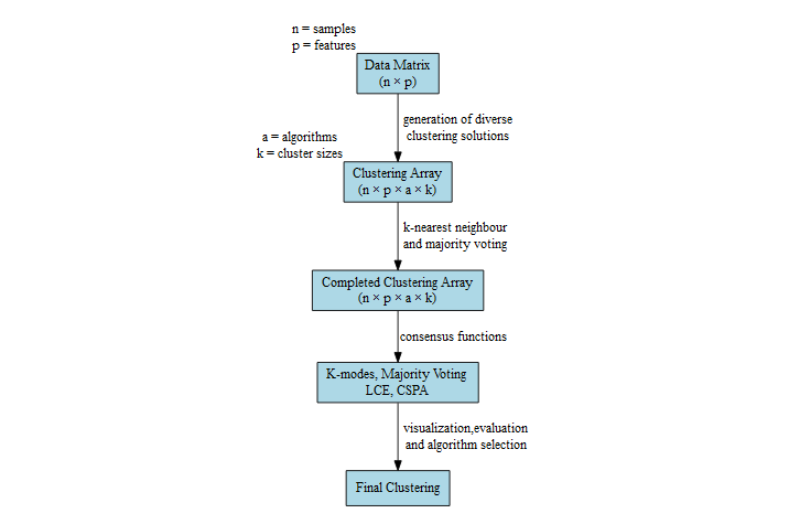
The goal of diceR is to provide a systematic framework for generating diverse cluster ensembles in R. There are a lot of nuances in cluster analysis to consider. We provide a process and a suite of functions and tools to implement a systematic framework for cluster discovery, guiding the user through the generation of a diverse clustering solutions from data, ensemble formation, algorithm selection and the arrival at a final consensus solution. We have additionally developed visual and analytical validation tools to help with the assessment of the final result. We implemented a wrapper function dice() that allows the user to easily obtain results and assess them. Thus, the package is accessible to both end user with limited statistical knowledge. Full access to the package is available for informaticians and statisticians and the functions are easily expanded. More details can be found in our companion paper published at BMC Bioinformatics.

Installation

You can install diceR from CRAN with:

install.packages("diceR")

Or get the latest development version from GitHub:

# install.packages("devtools")
devtools::install_github("AlineTalhouk/diceR")

Example

The following example shows how to use the main function of the package, dice(). A data matrix hgsc contains a subset of gene expression measurements of High Grade Serous Carcinoma Ovarian cancer patients from the Cancer Genome Atlas publicly available datasets. Samples as rows, features as columns. The function below runs the package through the dice() function. We specify (a range of) nk clusters over reps subsamples of the data containing 80% of the full samples. We also specify the clustering algorithms to be used and the ensemble functions used to aggregated them in cons.funs.

library(diceR)
data(hgsc)
obj <- dice(hgsc, nk = 4, reps = 5, algorithms = c("hc", "diana"),
            cons.funs = c("kmodes", "majority"))

The first few cluster assignments are shown below:

knitr::kable(head(obj$clusters))

	kmodes	majority
TCGA.04.1331_PRO.C5	2	2
TCGA.04.1332_MES.C1	2	2
TCGA.04.1336_DIF.C4	4	2
TCGA.04.1337_MES.C1	2	2
TCGA.04.1338_MES.C1	2	2
TCGA.04.1341_PRO.C5	2	2

You can also compare the base algorithms with the cons.funs using internal evaluation indices:

knitr::kable(obj$indices$ii$`4`)

	Algorithms	calinski_harabasz	dunn	gamma	c_index	davies_bouldin	sd	s_dbw	silhouette	Compactness	Connectivity
HC_Euclidean	HC_Euclidean	3.104106	0.2608547	0.6349401	0.2844073	1.839182	2.846480	1.678968	-0.1418603	24.83225	41.62183
DIANA_Euclidean	DIANA_Euclidean	53.647400	0.3348103	-1.9749903	0.1589442	2.824201	3.450173	1.809561	0.0564065	21.93396	241.66310
kmodes	kmodes	55.138600	0.3396909	-1.8704101	0.1453599	2.006752	3.986950	1.967467	0.1369288	21.91494	201.42540
majority	majority	19.373248	0.3544371	0.6529653	0.2102487	1.622799	4.039708	1.982210	0.1504666	23.85408	64.04921

Pipeline

This figure is a visual schematic of the pipeline that dice() implements.

Ensemble Clustering pipeline.

Please visit the overview page for more detail.